Working with MikroTik and IP Infusion’s OcNOS to interop EVPN/VxLAN has been on my wish list for a long time. Both solutions are a great cost-effective alternative to mainstream vendors – both separately and together – for WISP/FISP/DC & Enterprise networks.
BGP EVPN and VxLAN
One of the more interesting trends to come out for the 2010s in network engineering was the rise of overlays in data center and enterprise networking. While carriers have been using MPLS and the various overlays available for that type of data plane since the early 2000s, enterprises and data centers tended to steer away from MPLS due to cost and complexity.
BGP EVPN – BGP Ethernet VPN or EVPN was originally designed for an MPLS data plane in RFC7432 and later modified to work with a VxLAN data plane in RFC8365.
It solves the following problems:
- Provides a control plane for VxLAN overlays
- Supports L2/L3 multitenancy via exchange of MAC addresses & IPv4/IPv6 routing inside of VRFs
- Multihoming at the Network Virtualization Edge (NVE)
- Multicast traffic in VxLAN overlays
VxLAN – VxLAN was developed in the early 2010s as an open-source alternative to Cisco’s OTV and released as RFC7348
Problems VxLAN solves:
- Scales beyond 4094 VLANs by using a 24-bit VxLAN Network Identifier or VNI (that can also be tied to a VLAN)
- Encapsulates ethernet frames inside of UDP
- Creates L2 domains for DC, Enterprise and even Service Provider use cases.
EVPN/VxLAN – Better together
VxLAN on its own was limited because it needed a control plane to dynamically create tunnels and manage MAC address learning. EVPN and VxLAN became popular because together, they allowed network operators to solve many of the same problems as MPLS with overlays but didn’t need every hop in the network to support a specific protocol as VxLAN works with standard IPv4/IPv6 headers so it can pass through routers and switches that don’t support VxLAN.
This created a migration opportunity for data centers and enterprises to leverage EVPN/VxLAN designs over time without a massive rip/replace of hardware.
Adding EVPN and VxLAN to RouterOS 7.
VxLAN

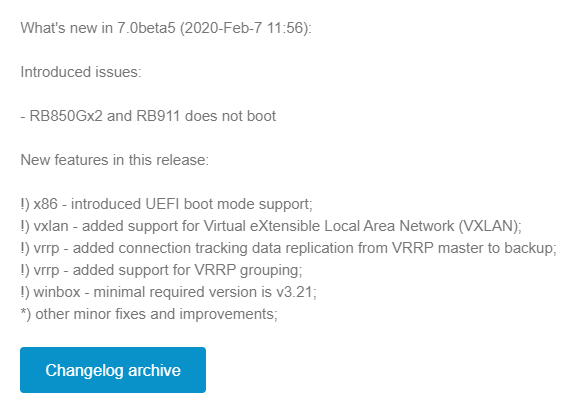
While IP Infusion has supported both of these in OcNOS for quite a while, pairing these features together in ROSv7 has been a long time in the making. VxLAN was added fairly early in RouterOS v7 beta in February 2020.
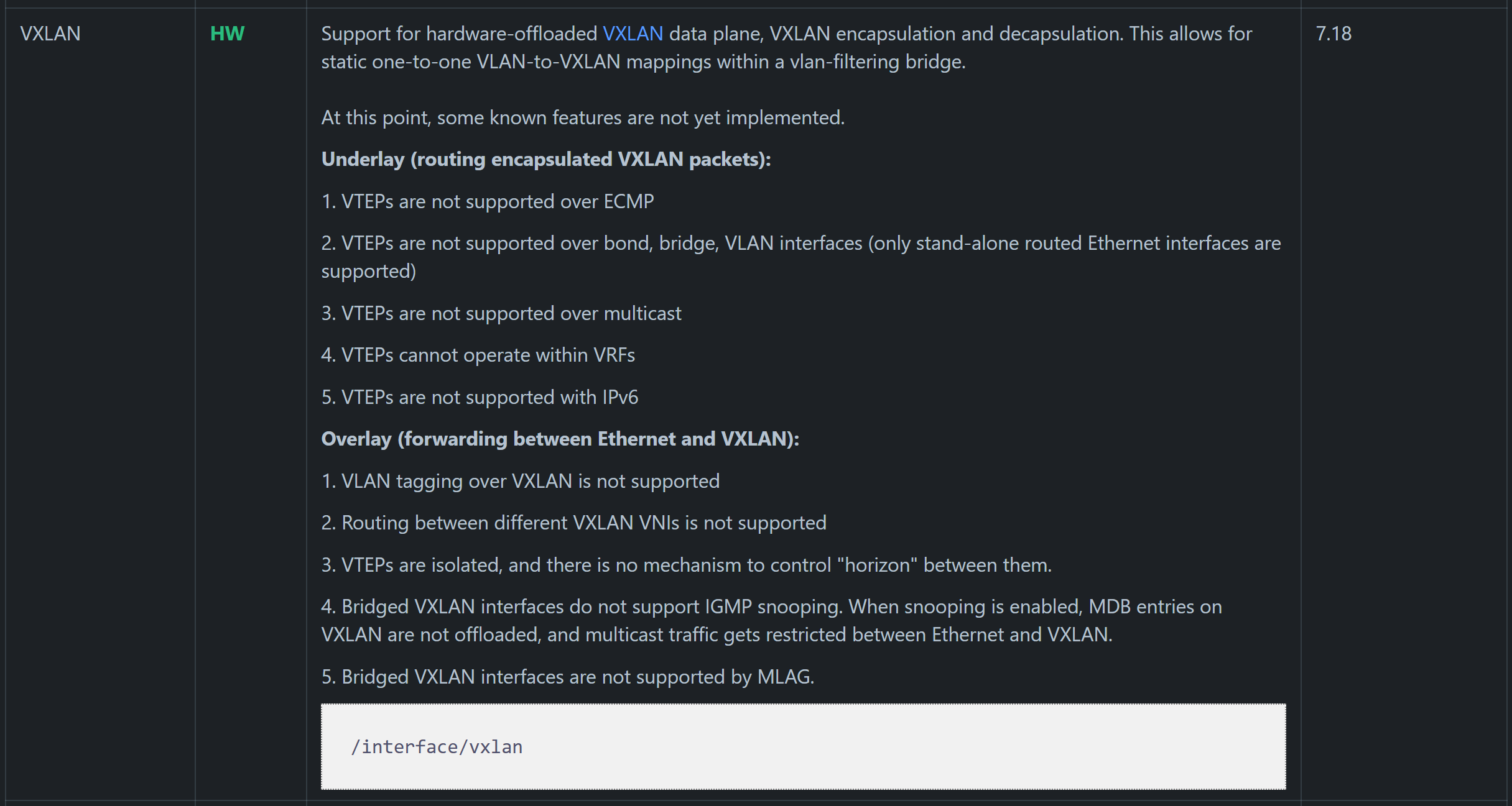
A newer addition to the VxLAN implementation in ROSv7 allows for the hardware offload of very simple network topologies in supported hardware. It has a number of caveats that make it unlikely to be used outside of a lab until more features are added but the potential is easy to see – low cost EVPN/VxLAN endpoints that can handle traffic at wirespeed in an ASIC.
BGP EVPN
BGP EVPN on the other hand was a more recent addition in ROSv7.20beta2
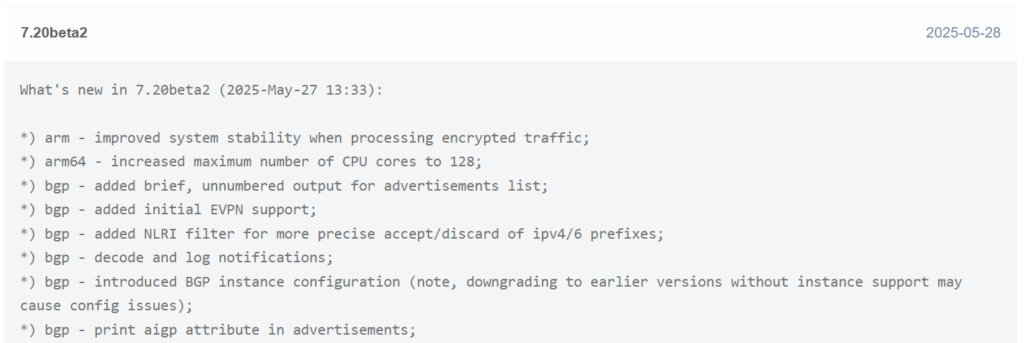
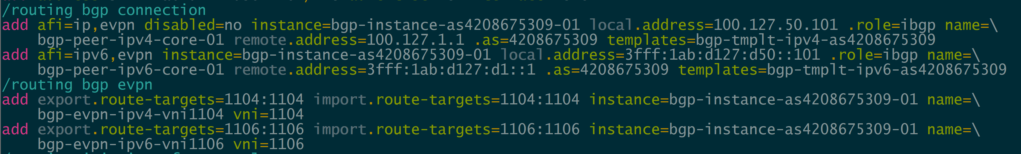
MikroTik added the EVPN address family to BGP peerings and the ability to set import/export route targets per VNI and BGP instance.
There are five EVPN route types defined:
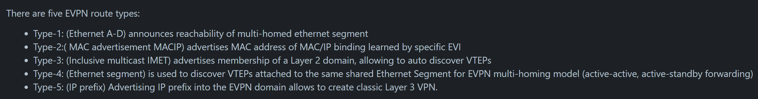
MikroTik has currently implemented Type 3 IMET routes:
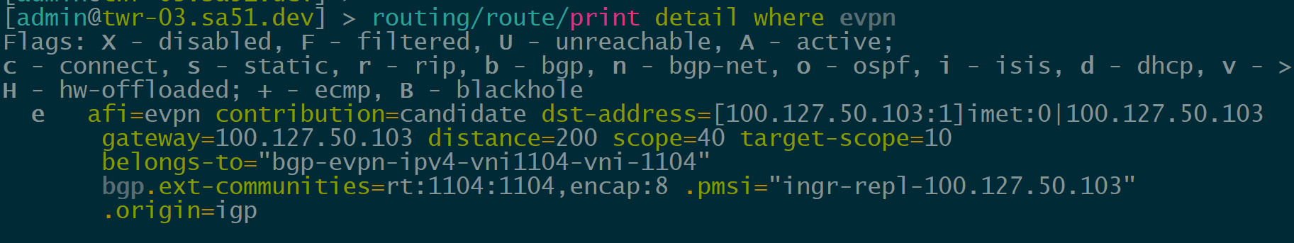
However, RouterOS can learn and display other EVPN route types like macip (though it may not be able to fully utilize all of them)
Given the amount of effort MikroTik has recently put into EVPN and VxLAN hw offload, it seems reasonable that we’ll see other EVPN route types and hardware capabilities enabled.
EVE-NG lab concept and overview
Topology
While EVPN/VxLAN is more often used in the data center or within enterprises, it’s sometimes used in service providers as well. Though it’s more common to see EVPN with an MPLS data plane in the ISP world.
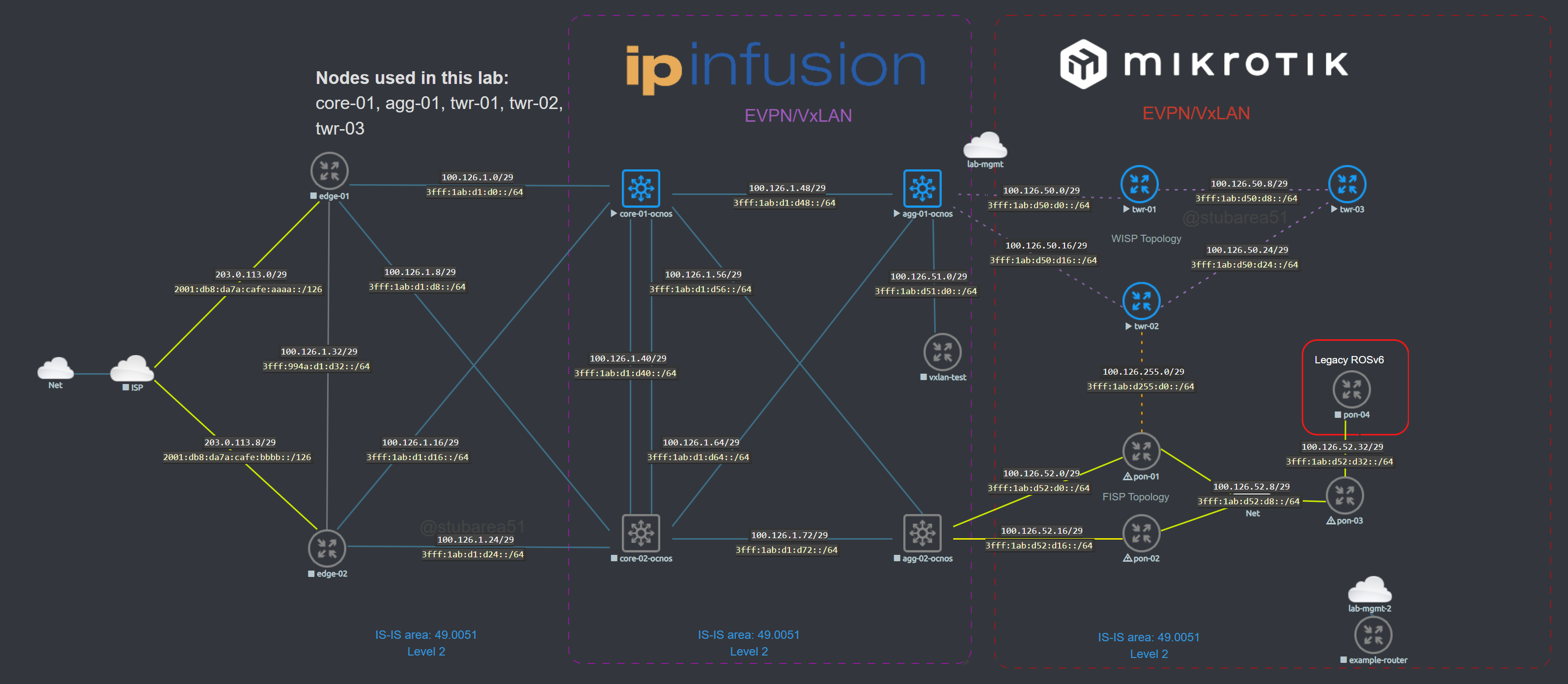
The lab topology is based on a WISP/FISP design and is one i’ve been using for a while to test a number of different features, designs and operating systems.
Nodes used
For this lab, we’ll be using the core-01, agg-01 and twr-01, 02 and 03 nodes (blue nodes are powered on).
IS-IS Underlay
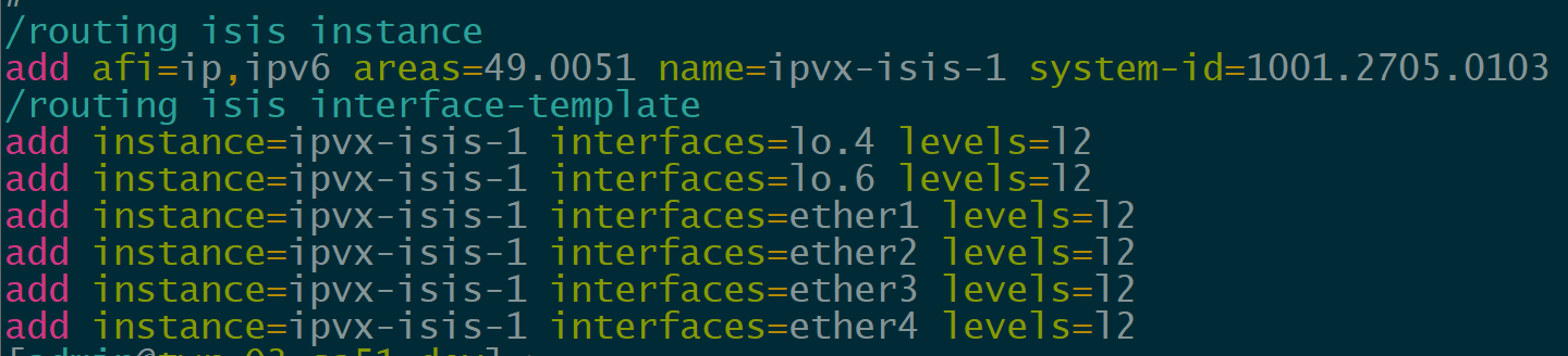
In order to provide reachability for iBGP, we are using IS-IS as the IGP for several reasons.
- Highly scalable and stable
- IPv4/IPv6 using the same instance
- Does not have the same area design constraints as OSPF
IP Infusion OcNOS has supported IS-IS for quite a while but it’s a newer addition to MikroTik with support added in ROSv7.13.
If you want to learn more about using IS-IS in RouterOS, I presented an overview of the protocol at the MikroTik Professionals Conference in 2024.
IPv4 and IPv6
Most of my labs are dual-stack or single stack IPv6 unless the feature or protocol i’m testing is IPv4 only.
IPv6 transition continues to increase and it’s important to test with the newest version of the Internet protocol whenever possible.
This lab utilizes RFC9637 IPv6 space because it allows us to model a variety of network types from a single ISP to a mock-up of the entire IPv6 Internet if desired.
3fff::/20OcNOS as a BGP EVPN route reflector
Since MikroTik has one EVPN route type working and only supports ETREE leaf type, I ended up using OcNOS SP as a BGP route reflector for IPv4, IPv6 and EVPN AFIs.
As EVPN support improves, i’ll update the testing to include using VTEPs between OcNOS and RouterOS.
Lab Validation
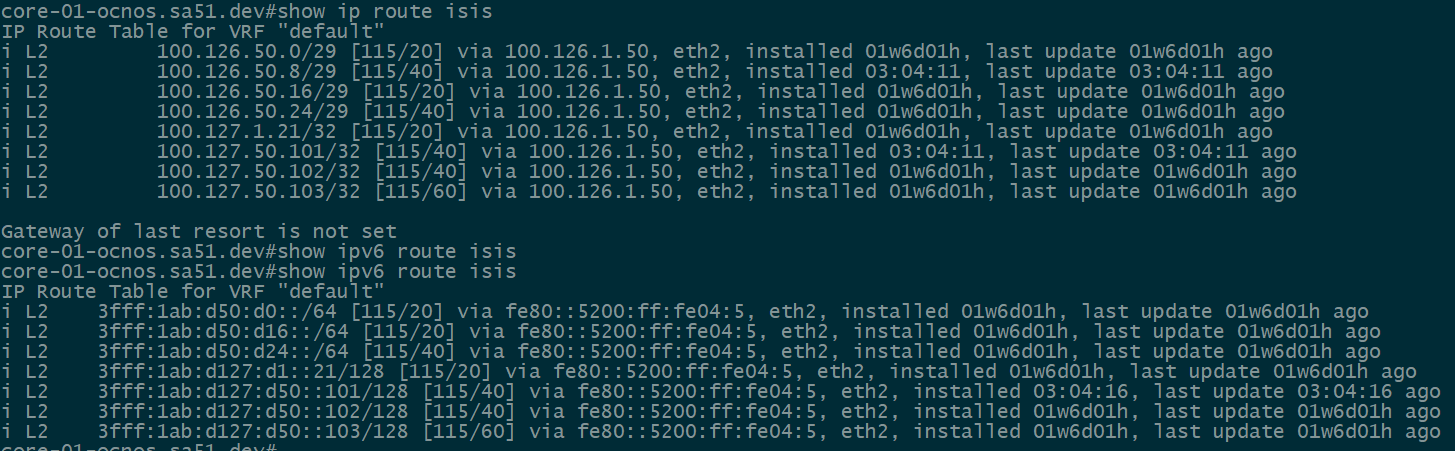
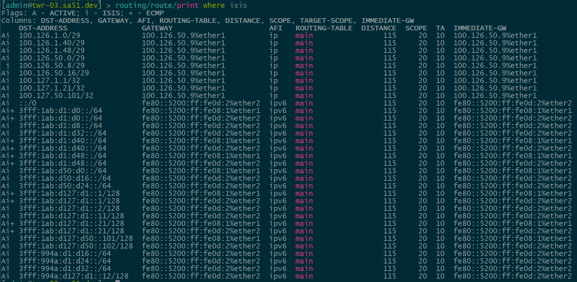
IS-IS underlay
Our first step is to validate IPv4 and IPv6 IS-IS routes between the core and the towers. All of the loopback and ptp routes between the core and towers show up and are reachable.
core-01
twr-03
BGP Peerings
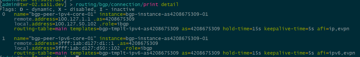
Next, we want to ensure that BGP peerings are up between the towers and the RR. We can see established peerings on both IPv4 and IPv6 loopbacks to all towers.
core-01
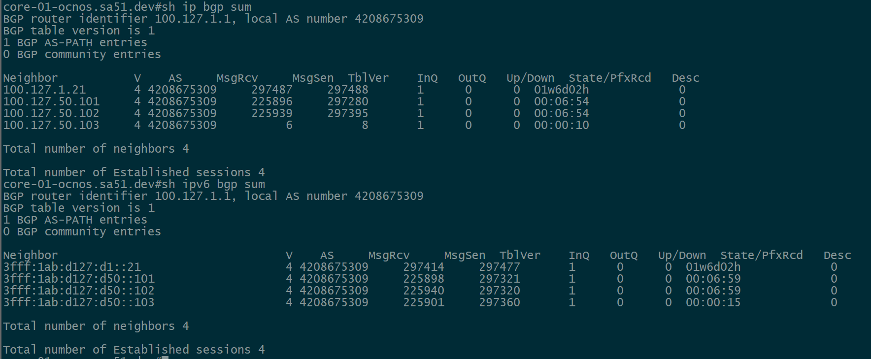
twr-02
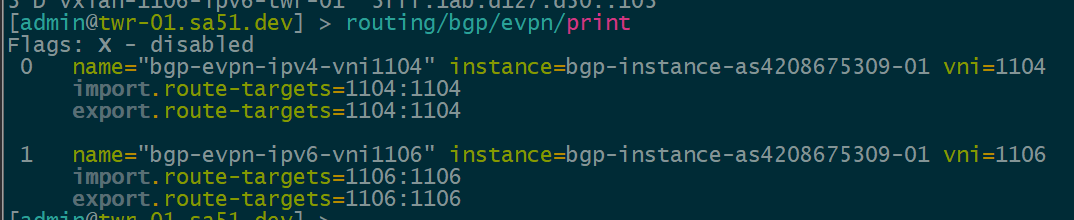
BGP EVPN VNI and Route Target Import/Export configured
In order to create the dynamic VTEPS in VxLAN for a VNI, we have to create the correct EVPN configuration for the VNIs we are going to use as well as route target import & export
twr-01
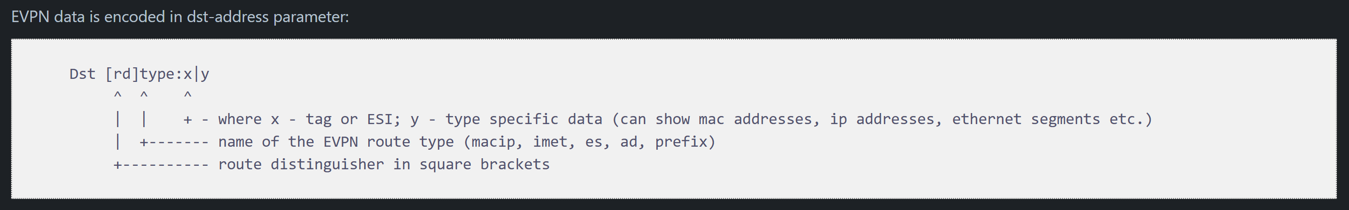
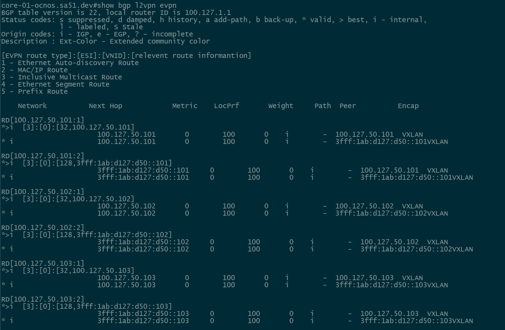
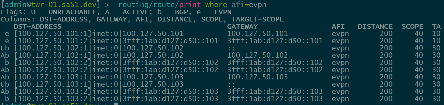
BGP EVPN Routes advertised and learned
Now let’s validate that EVPN routes are being reflected and learned between the towers and the RR. Based on the output, we see multiple EVPN Type 3 routes with a next hop to each of the three tower loopbacks for IPv4 and IPv6.
core-01
twr-01
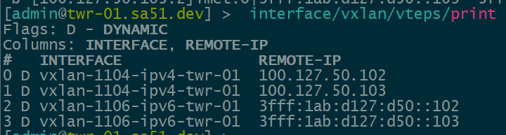
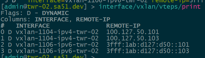
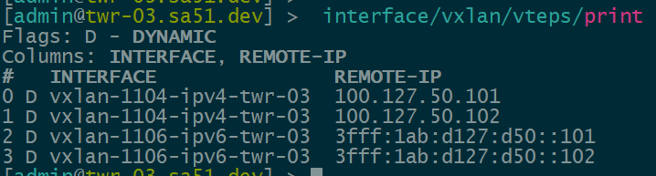
Dynamic VTEPs created
Now that EVPN is working and exchanging information on the VNIs we have configured, we can see the VTEPS have ben automatically created over both IPv4 and IPv6 and each tower can reach the other within the VNIs.
twr-01
twr-02
twr-03
Overlay Reachability
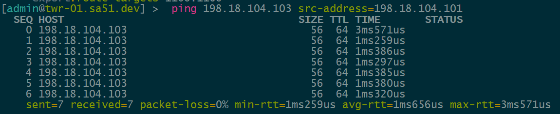
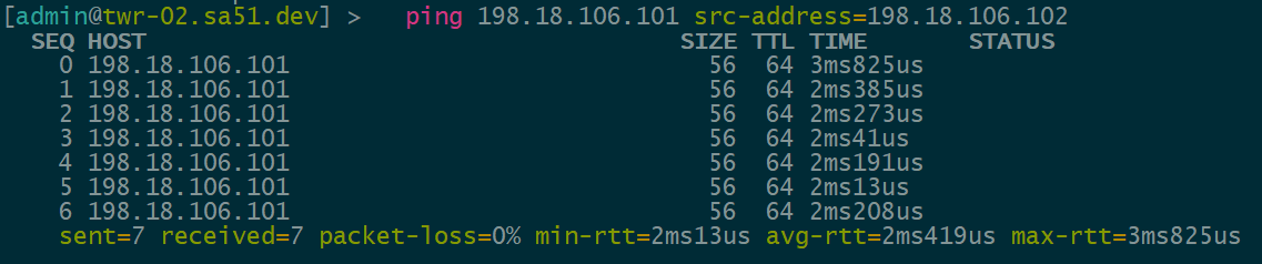
The final validation is to check and see if the IPv4 addresses configured over each type of VTEP can reach each other within the overlay.
VNI 1104 is tied to VLAN1104 for IPv4 VTEPs and uses 198.18.104.0/24
VNI 1106 is tied to VLAN1106 for IPv6 VTEPs and uses 198.18.106.0/24
IPv4 over IPv4 EVPN/VxLAN – twr-01 to twr-03
IPv4 over IPv6 EVPN/VxLAN – twr-02 to twr-01
Lab configurations
OcNOS VM for EVE-NG can be downloaded here:
MikroTik CHR VM can be downloaded here:
EVE-NG can be downloaded here:
core-01-ocnos.sa51.dev
! Software version: DEMO_VM-OcNOS-SP-PLUS-x86-6.6.0.248-GA 03/24/2025 05:49:09
!
! No configuration change since last reboot
!
feature netconf-ssh
feature netconf-tls
!
service password-encryption
!
snmp-server enable traps link linkDown
snmp-server enable traps link linkUp
!
bgp extended-asn-cap
!
qos enable
!
hostname core-01-ocnos.sa51.dev
no ip domain-lookup
errdisable cause stp-bpdu-guard
feature telnet vrf management
feature dns relay
ip dns relay
ipv6 dns relay
feature ntp vrf management
ntp enable vrf management
!
nvo vxlan enable
!
ip vrf management
!
interface po1
 description core-01-to-core-02
 shutdown
 ip router isis sa51
 ipv6 router isis sa51
!
interface lo
 ip address 127.0.0.1/8
 ip address 100.127.1.1/32 secondary
 ipv6 address ::1/128
 ipv6 address 3fff:1ab:d127:d1::1/128
 ip router isis sa51
 ipv6 router isis sa51
!
interface eth0
 ip vrf forwarding management
 ip address dhcp
 ipv6 address autoconfig
!
interface eth1
!
interface eth2
 description core-01-to-agg-01
 ip address 100.126.1.49/29
 ipv6 address 3fff:1ab:d1:d48::49/64
 ip router isis sa51
 ipv6 router isis sa51
!
interface eth3
!
interface eth4
 description core-01-to-core-02
 ip address 100.126.1.41/29
 ipv6 address 3fff:1ab:d1:d40::41/64
 ip router isis sa51
 ipv6 router isis sa51
!
interface eth5
 description core-01-to-core-02
 shutdown
!
interface eth6
 description to-edge-01
 ip address 100.126.1.1/29
 ipv6 address 3fff:1ab:d1:d0::1/64
 ip router isis sa51
 ipv6 router isis sa51
!
interface eth7
!
 exit
!
router isis sa51
 is-type level-2-only
 metric-style wide
 net 49.0051.1001.2700.1001.00
!
router bgp 4208675309
 bgp router-id 100.127.1.1
 no bgp inbound-route-filter
 neighbor bgp-pg-ipv4-as4208675309 peer-group
 neighbor bgp-pg-ipv4-as4208675309 remote-as 4208675309
 neighbor bgp-pg-ipv4-as4208675309 update-source lo
 neighbor bgp-pg-ipv4-as4208675309 timers 5 15
 neighbor bgp-pg-ipv6-as4208675309 peer-group
 neighbor bgp-pg-ipv6-as4208675309 remote-as 4208675309
 neighbor bgp-pg-ipv6-as4208675309 update-source lo
 neighbor bgp-pg-ipv6-as4208675309 timers 5 15
 neighbor 100.127.1.21 peer-group bgp-pg-ipv4-as4208675309
 neighbor 100.127.50.101 peer-group bgp-pg-ipv4-as4208675309
 neighbor 100.127.50.102 peer-group bgp-pg-ipv4-as4208675309
 neighbor 100.127.50.103 peer-group bgp-pg-ipv4-as4208675309
 neighbor 3fff:1ab:d127:d1::21 peer-group bgp-pg-ipv6-as4208675309
 neighbor 3fff:1ab:d127:d50::101 peer-group bgp-pg-ipv6-as4208675309
 neighbor 3fff:1ab:d127:d50::102 peer-group bgp-pg-ipv6-as4208675309
 neighbor 3fff:1ab:d127:d50::103 peer-group bgp-pg-ipv6-as4208675309
 !
 address-family ipv4 unicast
 neighbor bgp-pg-ipv4-as4208675309 activate
 neighbor bgp-pg-ipv4-as4208675309 route-reflector-client
 exit-address-family
 !
 address-family l2vpn evpn
 neighbor bgp-pg-ipv4-as4208675309 activate
 neighbor bgp-pg-ipv4-as4208675309 route-reflector-client
 neighbor bgp-pg-ipv6-as4208675309 activate
 neighbor bgp-pg-ipv6-as4208675309 route-reflector-client
 exit-address-family
 !
 address-family ipv6 unicast
 neighbor bgp-pg-ipv6-as4208675309 activate
 neighbor bgp-pg-ipv6-as4208675309 route-reflector-client
 exit-address-family
 !
 exit
!
!
agg-01-ocnos.sa51.dev
! Software version: DEMO_VM-OcNOS-SP-PLUS-x86-6.6.0.248-GA 03/24/2025 05:49:09
!
! No configuration change since last reboot
!
feature netconf-ssh
feature netconf-tls
!
service password-encryption
!
snmp-server enable traps link linkDown
snmp-server enable traps link linkUp
!
bgp extended-asn-cap
!
qos enable
!
hostname agg-01-ocnos.sa51.dev
no ip domain-lookup
bridge 1 protocol ieee vlan-bridge
errdisable cause stp-bpdu-guard
data-center-bridging enable bridge 1
feature telnet vrf management
feature dns relay
ip dns relay
ipv6 dns relay
feature ntp vrf management
ntp enable vrf management
!
vlan database
 vlan 101 bridge 1 state enable
!
nvo vxlan enable
!
ip vrf management
!
mac vrf vrf-evpn-1101
 rd 100.127.1.21:1101
 route-target both evpn-auto-rt
!
nvo vxlan vtep-ip-global 100.127.1.21
!
interface lo
 ip address 127.0.0.1/8
 ip address 100.127.1.21/32 secondary
 ipv6 address ::1/128
 ipv6 address 3fff:1ab:d127:d1::21/128
 ip router isis sa51
 ipv6 router isis sa51
!
interface eth0
 ip vrf forwarding management
 ip address dhcp
 ipv6 address autoconfig
!
interface eth1
!
interface eth2
 description agg-01-to-twr-01
 ip address 100.126.50.1/29
 ipv6 address 3fff:1ab:d50:d0::1/64
 ip router isis sa51
 ipv6 router isis sa51
!
interface eth3
 description agg-01-to-twr-02
 ip address 100.126.50.17/29
 ipv6 address 3fff:1ab:d50:d16::d17/64
 ip router isis sa51
 ipv6 router isis sa51
!
interface eth4
 switchport
 bridge-group 1
!
interface eth5
 description agg-01-to-core-01
 ip address 100.126.1.50/29
 ipv6 address 3fff:1ab:d1:d48::50/64
 ip router isis sa51
 ipv6 router isis sa51
!
interface eth6
!
interface eth7
!
 exit
!
router isis sa51
 is-type level-2-only
 metric-style wide
 net 49.0051.1001.2700.1021.00
!
router bgp 4208675309
 bgp router-id 100.127.1.21
 no bgp inbound-route-filter
 neighbor bgp-pg-ipv4-as4208675309 peer-group
 neighbor bgp-pg-ipv4-as4208675309 remote-as 4208675309
 neighbor bgp-pg-ipv4-as4208675309 update-source lo
 neighbor bgp-pg-ipv4-as4208675309 timers 5 15
 neighbor bgp-pg-ipv6-as4208675309 peer-group
 neighbor bgp-pg-ipv6-as4208675309 remote-as 4208675309
 neighbor bgp-pg-ipv6-as4208675309 update-source lo
 neighbor bgp-pg-ipv6-as4208675309 timers 5 15
 neighbor 100.127.1.1 peer-group bgp-pg-ipv4-as4208675309
 neighbor 3fff:1ab:d127:d1::1 peer-group bgp-pg-ipv6-as4208675309
 !
 address-family ipv4 unicast
 neighbor bgp-pg-ipv4-as4208675309 activate
 neighbor bgp-pg-ipv4-as4208675309 route-reflector-client
 exit-address-family
 !
 address-family l2vpn evpn
 neighbor bgp-pg-ipv4-as4208675309 activate
 neighbor bgp-pg-ipv4-as4208675309 route-reflector-client
 neighbor bgp-pg-ipv6-as4208675309 activate
 exit-address-family
 !
 address-family ipv6 unicast
 neighbor bgp-pg-ipv6-as4208675309 activate
 exit-address-family
 !
 exit
!
!
end
twr-01.sa51.dev
/interface bridge
add name=br-router vlan-filtering=yes
add name=lo.4
add name=lo.6
/interface ethernet
set [ find default-name=ether1 ] disable-running-check=no
set [ find default-name=ether2 ] disable-running-check=no
set [ find default-name=ether3 ] disable-running-check=no
set [ find default-name=ether4 ] disable-running-check=no
set [ find default-name=ether5 ] disable-running-check=no
set [ find default-name=ether6 ] disable-running-check=no
set [ find default-name=ether7 ] disable-running-check=no
set [ find default-name=ether8 ] disable-running-check=no
/interface vxlan
add bridge=br-router bridge-pvid=1104 learning=no local-address=100.127.50.101 mac-address=72:F8:A7:93:B5:43 name=vxlan-1104-ipv4-twr-01 vni=1104
add bridge=br-router bridge-pvid=1106 learning=no local-address=3fff:1ab:d127:d50::101 mac-address=0E:2C:97:B8:5F:8D name=vxlan-1106-ipv6-twr-01 vni=1106 \
    vteps-ip-version=ipv6
/interface vlan
add interface=br-router name=v1104 vlan-id=1104
add interface=br-router name=v1106 vlan-id=1106
/ip vrf
add interfaces=ether8 name=vrf-lab-mgmt
/port
set 0 name=serial0
/routing bgp instance
add as=4208675309 name=bgp-instance-as4208675309-01 router-id=100.127.50.101
/routing bgp template
add afi=ip as=4208675309 hold-time=15s keepalive-time=5s name=bgp-tmplt-ipv4-as4208675309
add afi=ipv6 as=4208675309 hold-time=15s keepalive-time=5s name=bgp-tmplt-ipv6-as4208675309
/routing id
add disabled=no id=100.127.50.101 name=id-main select-dynamic-id=""
/routing isis instance
add afi=ip,ipv6 areas=49.0051 l2.originate-default=never name=ipvx-isis-1 system-id=1001.2705.0101
/ipv6 settings
set accept-router-advertisements=yes
/interface bridge vlan
add bridge=br-router tagged=br-router vlan-ids=1106
add bridge=br-router tagged=br-router vlan-ids=1104
/ip address
add address=100.126.50.2/29 interface=ether1 network=100.126.50.0
add address=100.127.50.101 interface=lo.4 network=100.127.50.101
add address=100.126.50.9/29 interface=ether2 network=100.126.50.8
add address=198.18.106.101/24 interface=v1106 network=198.18.106.0
add address=198.18.104.101/24 interface=v1104 network=198.18.104.0
/ip dhcp-client
add interface=ether8
/ipv6 route
add gateway=3fff:da7a:1ab:77::1 routing-table=vrf-lab-mgmt vrf-interface=vrf-lab-mgmt
/ip service
set ssh vrf=vrf-lab-mgmt
set winbox vrf=vrf-lab-mgmt
/ipv6 address
add address=3fff:1ab:d127:d50::101/128 advertise=no interface=lo.6
/routing bgp connection
add afi=ip,evpn disabled=no instance=bgp-instance-as4208675309-01 local.address=100.127.50.101 .role=ibgp name=bgp-peer-ipv4-core-01 remote.address=100.127.1.1 \
    .as=4208675309 templates=bgp-tmplt-ipv4-as4208675309
add afi=ipv6,evpn instance=bgp-instance-as4208675309-01 local.address=3fff:1ab:d127:d50::101 .role=ibgp name=bgp-peer-ipv6-core-01 remote.address=\
    3fff:1ab:d127:d1::1 .as=4208675309 templates=bgp-tmplt-ipv6-as4208675309
/routing bgp evpn
add export.route-targets=1104:1104 import.route-targets=1104:1104 instance=bgp-instance-as4208675309-01 name=bgp-evpn-ipv4-vni1104 vni=1104
add export.route-targets=1106:1106 import.route-targets=1106:1106 instance=bgp-instance-as4208675309-01 name=bgp-evpn-ipv6-vni1106 vni=1106
/routing isis interface-template
add instance=ipvx-isis-1 interfaces=lo.4 levels=l2
add instance=ipvx-isis-1 interfaces=lo.6 levels=l2
add instance=ipvx-isis-1 interfaces=ether1 levels=l2
add instance=ipvx-isis-1 interfaces=ether2 levels=l2
add instance=ipvx-isis-1 interfaces=ether3 levels=l2
add instance=ipvx-isis-1 interfaces=ether4 levels=l2
/system identity
set name=twr-01.sa51.dev
/system note
set show-at-login=no
/tool romon
set enabled=yes
/tool sniffer
set file-limit=10000KiB file-name=bgp-twr-01 filter-ip-protocol=tcp filter-port=bgp
twr-02.sa51.dev
/interface bridge
add name=br-router vlan-filtering=yes
add name=lo.4
add name=lo.6
/interface ethernet
set [ find default-name=ether1 ] disable-running-check=no
set [ find default-name=ether2 ] disable-running-check=no
set [ find default-name=ether3 ] disable-running-check=no
set [ find default-name=ether4 ] disable-running-check=no
set [ find default-name=ether5 ] disable-running-check=no
set [ find default-name=ether6 ] disable-running-check=no
set [ find default-name=ether7 ] disable-running-check=no
set [ find default-name=ether8 ] disable-running-check=no
/interface vxlan
add bridge=br-router bridge-pvid=1104 learning=no local-address=100.127.50.102 mac-address=EA:DC:97:20:66:1D name=vxlan-1104-ipv4-twr-02 vni=\
    1104
add bridge=br-router bridge-pvid=1106 learning=no local-address=3fff:1ab:d127:d50::102 mac-address=12:37:A4:64:42:DD name=vxlan-1106-ipv6-twr-02 \
    vni=1106 vteps-ip-version=ipv6
/interface vlan
add interface=br-router name=v1104 vlan-id=1104
add interface=br-router name=v1106 vlan-id=1106
/ip vrf
add interfaces=ether8 name=vrf-lab-mgmt
/port
set 0 name=serial0
/routing bgp instance
add as=4208675309 name=bgp-instance-as4208675309-01 router-id=100.127.50.102
/routing bgp template
add afi=ip as=4208675309 hold-time=15s keepalive-time=5s name=bgp-tmplt-ipv4-as4208675309
add afi=ipv6 as=4208675309 hold-time=15s keepalive-time=5s name=bgp-tmplt-ipv6-as4208675309
/routing id
add disabled=no id=100.127.50.102 name=id-main select-dynamic-id=""
/routing isis instance
add afi=ip,ipv6 areas=49.0051 l2.originate-default=never name=ipvx-isis-1 system-id=1001.2705.0102
/ipv6 settings
set accept-router-advertisements=yes
/interface bridge vlan
add bridge=br-router tagged=br-router vlan-ids=1106
add bridge=br-router tagged=br-router vlan-ids=1104
/ip address
add address=100.126.50.18/29 interface=ether1 network=100.126.50.16
add address=100.127.50.102 interface=lo.4 network=100.127.50.102
add address=100.126.50.25/29 interface=ether3 network=100.126.50.24
add address=198.18.106.102/24 interface=v1106 network=198.18.106.0
add address=198.18.104.102/24 interface=v1104 network=198.18.104.0
/ip dhcp-client
add interface=ether8
/ipv6 route
add gateway=3fff:da7a:1ab:77::1 routing-table=vrf-lab-mgmt vrf-interface=vrf-lab-mgmt
/ip service
set ssh vrf=vrf-lab-mgmt
set winbox vrf=vrf-lab-mgmt
/ipv6 address
add address=3fff:1ab:d127:d50::102/128 advertise=no interface=lo.6
add address=3fff:1ab:d50:d16::d18 advertise=no interface=ether1
add address=3fff:1ab:d50:d24::d25 advertise=no interface=ether3
/routing bgp connection
add afi=ip,evpn disabled=no instance=bgp-instance-as4208675309-01 local.address=100.127.50.102 .role=ibgp name=bgp-peer-ipv4-core-01 \
    remote.address=100.127.1.1 .as=4208675309 templates=bgp-tmplt-ipv4-as4208675309
add afi=ipv6,evpn instance=bgp-instance-as4208675309-01 local.address=3fff:1ab:d127:d50::102 .role=ibgp name=bgp-peer-ipv6-core-01 \
    remote.address=3fff:1ab:d127:d1::1 .as=4208675309 templates=bgp-tmplt-ipv6-as4208675309
/routing bgp evpn
add export.route-targets=1104:1104 import.route-targets=1104:1104 instance=bgp-instance-as4208675309-01 name=bgp-evpn-ipv4-vni1104 vni=1104
add export.route-targets=1106:1106 import.route-targets=1106:1106 instance=bgp-instance-as4208675309-01 name=bgp-evpn-ipv6-vni1106 vni=1106
/routing isis interface-template
add instance=ipvx-isis-1 interfaces=lo.4 levels=l2
add instance=ipvx-isis-1 interfaces=lo.6 levels=l2
add instance=ipvx-isis-1 interfaces=ether1 levels=l2
add instance=ipvx-isis-1 interfaces=ether2 levels=l2
add instance=ipvx-isis-1 interfaces=ether3 levels=l2
add instance=ipvx-isis-1 interfaces=ether4 levels=l2
/system identity
set name=twr-02.sa51.dev
/system note
set show-at-login=no
/tool romon
set enabled=yes
twr-03.sa51.dev
/interface bridge
add name=br-router vlan-filtering=yes
add name=lo.4
add name=lo.6
/interface ethernet
set [ find default-name=ether1 ] disable-running-check=no
set [ find default-name=ether2 ] disable-running-check=no
set [ find default-name=ether3 ] disable-running-check=no
set [ find default-name=ether4 ] disable-running-check=no
set [ find default-name=ether5 ] disable-running-check=no
set [ find default-name=ether6 ] disable-running-check=no
set [ find default-name=ether7 ] disable-running-check=no
set [ find default-name=ether8 ] disable-running-check=no
/interface vxlan
add bridge=br-router bridge-pvid=1104 learning=no local-address=100.127.50.103 mac-address=8E:9A:2E:06:F9:A6 name=vxlan-1104-ipv4-twr-03 vni=\
    1104
add bridge=br-router bridge-pvid=1106 learning=no local-address=3fff:1ab:d127:d50::103 mac-address=BA:73:44:4C:51:5D name=vxlan-1106-ipv6-twr-03 \
    vni=1106 vteps-ip-version=ipv6
/interface vlan
add interface=br-router name=v1104 vlan-id=1104
add interface=br-router name=v1106 vlan-id=1106
/ip vrf
add interfaces=ether8 name=vrf-lab-mgmt
/port
set 0 name=serial0
/routing bgp template
add afi=ip as=4208675309 hold-time=15s keepalive-time=5s name=bgp-tmplt-ipv4-as4208675309
add afi=ipv6 as=4208675309 hold-time=15s keepalive-time=5s name=bgp-tmplt-ipv6-as4208675309
/routing id
add disabled=no id=100.127.50.103 name=id-main select-dynamic-id=""
/routing bgp instance
add as=4208675309 name=bgp-instance-as4208675309-01 router-id=id-main
/routing isis instance
add afi=ip,ipv6 areas=49.0051 name=ipvx-isis-1 system-id=1001.2705.0103
/ipv6 settings
set accept-router-advertisements=yes
/interface bridge vlan
add bridge=br-router tagged=br-router vlan-ids=1106
add bridge=br-router tagged=br-router vlan-ids=1104
/ip address
add address=100.126.50.10/29 interface=ether1 network=100.126.50.8
add address=100.127.50.103 interface=lo.4 network=100.127.50.103
add address=198.18.106.103/24 interface=v1106 network=198.18.106.0
add address=198.18.104.103/24 interface=v1104 network=198.18.104.0
/ip dhcp-client
add interface=ether8
/ipv6 route
add gateway=3fff:da7a:1ab:77::1 routing-table=vrf-lab-mgmt vrf-interface=vrf-lab-mgmt
/ip service
set ssh vrf=vrf-lab-mgmt
set winbox vrf=vrf-lab-mgmt
/ipv6 address
add address=3fff:1ab:d127:d50::103/128 advertise=no interface=lo.6
/routing bgp connection
add afi=ip,evpn disabled=no instance=bgp-instance-as4208675309-01 local.address=100.127.50.103 .role=ibgp name=bgp-peer-ipv4-core-01 \
    remote.address=100.127.1.1 .as=4208675309 templates=bgp-tmplt-ipv4-as4208675309
add afi=ipv6,evpn instance=bgp-instance-as4208675309-01 local.address=3fff:1ab:d127:d50::103 .role=ibgp name=bgp-peer-ipv6-core-01 \
    remote.address=3fff:1ab:d127:d1::1 .as=4208675309 templates=bgp-tmplt-ipv6-as4208675309
/routing bgp evpn
add export.route-targets=1104:1104 import.route-targets=1104:1104 instance=bgp-instance-as4208675309-01 name=bgp-evpn-ipv4-vni1104 vni=1104
add export.route-targets=1106:1106 import.route-targets=1106:1106 instance=bgp-instance-as4208675309-01 name=bgp-evpn-ipv6-vni1106 vni=1106
/routing isis interface-template
add instance=ipvx-isis-1 interfaces=lo.4 levels=l2
add instance=ipvx-isis-1 interfaces=lo.6 levels=l2
add instance=ipvx-isis-1 interfaces=ether1 levels=l2
add instance=ipvx-isis-1 interfaces=ether2 levels=l2
add instance=ipvx-isis-1 interfaces=ether3 levels=l2
add instance=ipvx-isis-1 interfaces=ether4 levels=l2
/system identity
set name=twr-03.sa51.dev
/system note
set show-at-login=no
/tool romon